 |
 |
 |
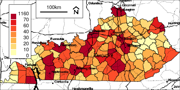 |
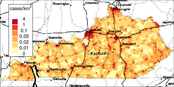
Figure 1: Events for Simulation 1
Friday 5 January 2018
The localEM package contains functions to implement the kernel smoothing local-EM algorithm1 of disease data aggregated to geographical regions. This algorithm provides an nonparametric alternative to the standard geospatial models, such as the Besag-York-Mollie (BYM) model2, for estimating spatial risk of areal disease data. With disease cases typically aggregated to highly coarse geographical regions (e.g., census counties, or census subdivisions), the local-EM method creates a tessellation of distinct regions by overlaying the map of these coarse regions with another map containing fine geographical regions (e.g., census tracts, census blocks, or census dissemination areas) of population data. This allows for the spatial risk to be estimated at a better resolution with the fine regions.
The methodology of this package is demonstrated on simulated lung cancer cases for the state of Kentucky, USA. The spatial polygons for the census counties and tracts of Kentucky are included with this package.
ncores = round(parallel::detectCores()/2)
cellsFine = 500
cellsCoarse = 20
nsim = 12
nxv = 6
Sbw = unique(round(
  exp(seq(log(4), log(35), len=15))
  )) * 1000
threshold = c(1.1, 1.25, 1.5)
Nboot = 100
path = '/store/highResLocalem/'
cacheDir = 'highResCache/'
figDir = 'highResFigure/'
specify number of grid cells for simulation
if(requireNamespace('RandomFields', quietly = TRUE)) {
  cellsSimulate = 200
} else {
  cellsSimulate = 100
}require('mapmisc', quietly=TRUE)
require('rgdal', quietly=TRUE)
data('kentuckyCounty', package = 'localEM')
data('kentuckyTract', package = 'localEM')
data('kMap', package = 'localEM')kMap = mapmisc::tonerToTrans(
mapmisc::openmap(kentuckyCounty, fact=1.6, path='stamen-toner'))Using the simLgcp() function from the geostatsp package, case locations are simulated with the log Gaussian Cox process (LGCP) and following parameters:
kentuckyOffset = geostatsp::spdfToBrick(
    kentuckyTract,
    geostatsp::squareRaster(kentuckyTract, cellsSimulate),
    pattern = '^expected$',
    logSumExpected = TRUE)

set.seed(0)
kCases = geostatsp::simLgcp(
    param = c(mean = 0, variance = 0.4^2, range = 120 * 1000, shape = 2),
    covariates = list(logExpected = kentuckyOffset),
    offset = 'logExpected', n = nsim)
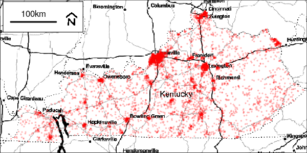
The simulated cases are then aggregated to the appropriate counties. Plots of the relative intensity, event locations and aggregated data are provided for the first simulated dataset.
kCases$agg = lapply(
    kCases[grep('^events[[:digit:]]+?', names(kCases))],
    function(qq) over(qq, kentuckyCounty)[,'id']
)

countyCounts = as.data.frame(lapply(
        kCases$agg,
        function(xx) {
          as.vector(table(xx, exclude = NULL)[
                  as.character(kentuckyCounty$id)])
        }
    ))

countyCounts[is.na(countyCounts)] = 0
names(countyCounts) = gsub('^events', 'count', names(countyCounts))
rownames(countyCounts) = as.character(kentuckyCounty$id)
kentuckyCounty = merge(kentuckyCounty, countyCounts, by.x = 'id', by.y = 'row.names') |
 |
 |
 |
Figure 1: Events for Simulation 1
The local-EM algorithm requires a smoothing parameter called the bandwidth to estimate the spatial risk. Small values of the bandwidth yield estimates similar to standardized incidence ratios of each areal regions, while large values yield estimates to the overall mean incidence ratio of the entire study area (i.e., [total counts]/[total offsets]). The preferred or optimal bandwidth for the disease data is one that minimizes the trade-off between the bias and variance of the estimator.
To automatic the selection of the optimal bandwidth, the lemXv() function of this package implements a likelihood cross-validation (CV) approach with the set of specified bandwidths. CV scores are computed with k-fold sampling without replacement of the dataset. The optimal bandwidth is the one that yields the smallest CV score.
The CV scores with 6-fold sampling are provided for the first simulated dataset.
library('localEM')

fileHere = file.path(path, 'xvKentucky.rds')

if(!file.exists(fileHere)) {

  xvKentucky = lemXv(
      cases = kentuckyCounty[,c('id','count1')],
      population = kentuckyTract,
      cellsCoarse = cellsCoarse,
      cellsFine = cellsFine,
      bw = Sbw,
      xv = nxv,
      ncores = ncores,
      path = path,
      verbose = TRUE)

  saveRDS(xvKentucky, file = fileHere)
} else {
  xvKentucky = readRDS(fileHere)
}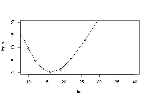 |
Figure 2: Cross-validation Scores for Simulation 1
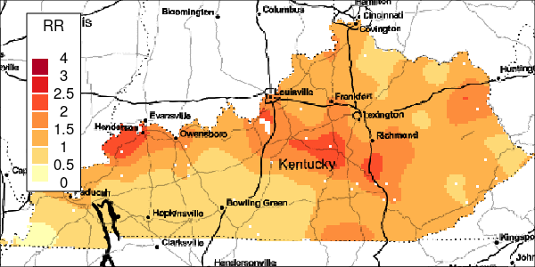
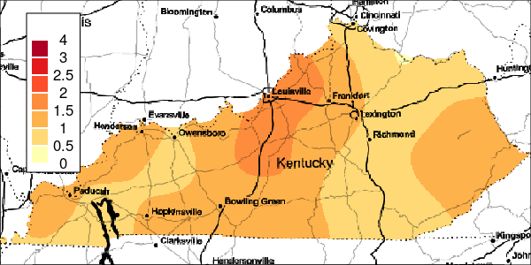
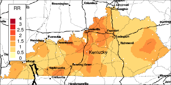
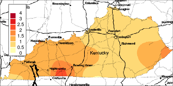
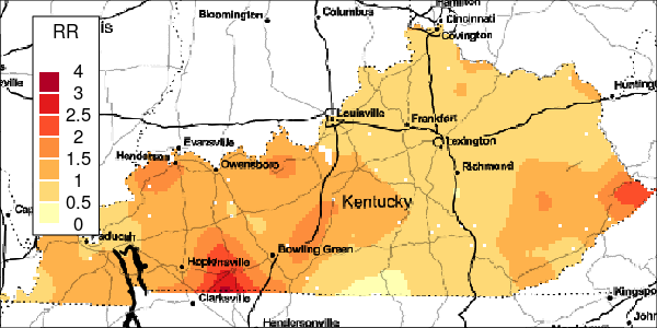
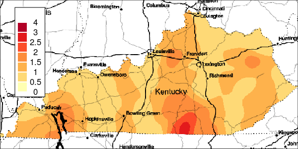
The R objects created from the lemXv() function also contain the local-EM risk estimation done with the optimal bandwidth found in the CV approach. High-resolution plots of the local-EM estimation with their optimal bandwidths are provided for all simulated datasets.
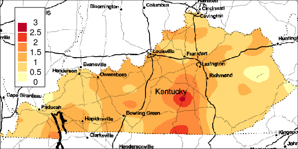
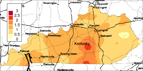
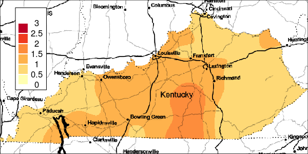
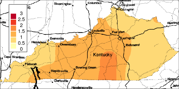
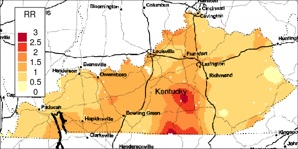
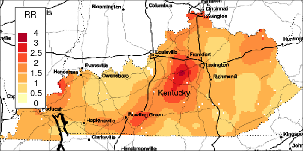
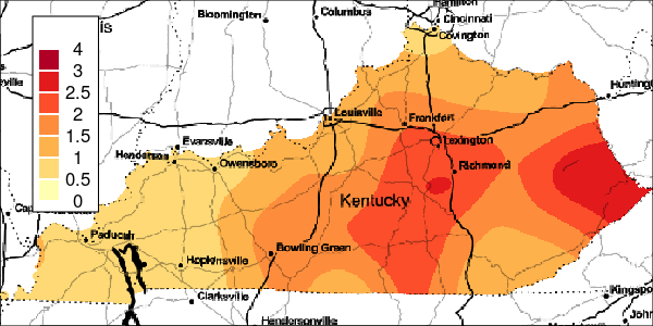
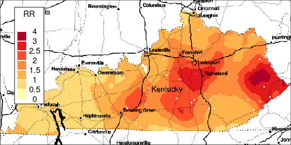
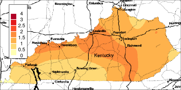
The riskEst() function allows local-EM risk estimation to be done with specified bandwidths. Plots of the local-EM estimation with all bandwidths used in this example are provided for the first simulated dataset. The plots show high cancer risk in the areas located east of Bowling Green and south of Frankfurt decreasing as the bandwidth increases.
riskKentucky = riskEst(
    cases = kentuckyCounty[,c('id','count1')],
    lemObjects = xvKentucky$smoothingMatrix,
    bw = Sbw,
    ncores = ncores,
    path = cacheDir)
## Loading required package: Matrix# estimated risk maps
toPlot = brick(filename(riskKentucky$riskEst))[[
round(seq(1, nlayers(riskKentucky$riskEst), len=6))
]]
SbwShort = as.numeric(gsub("^bw|_[[:alnum:]]+$", "", names(toPlot)))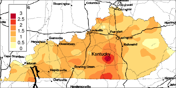 |
 |
 |
 |
 |
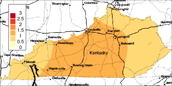 |
Figure 3: Risk Estimation for Simulation 1
To measure the uncertainty of the local-EM algorithm, the excProb() function computes the exceedance probabilities with the same bandwidth parameter used in the risk estimation. Bootstrapping from a Poisson process is used to simulate the events for calculating these exceedance probabilities.
Specifically, under the assumption that disease events are a realisation from the background population and constant risk threshold, cases are bootstrapped and randomly aggregated to the areal regions. Using the same bandwidth as the observed data, the local-EM risk is then estimated for each of the bootstrapped data. Afterwards, exceedance probabilities are computed as the proportion of the observed risk estimate at least as large as the ones of the bootstrap data. Large exceedance probabilities are consistent with the risk being greater than the specified threshold.
excProbKentucky = excProb(
    lemObjects = xvKentucky,
    threshold = threshold,
    Nboot = Nboot,
    fact = 2,
    ncores = ncores,
    path = path,
verbose=TRUE) |
 |
 |
 |
 |
Figure 4: Exceedance Probabilities for Simulation 1
Using the R objects created from the lemXv() function for the first simulated dataset, this CV method can be efficiently implemented on the remaining simulated datasets.
xvAllKentucky = lemXv(
    cases = kentuckyCounty@data[,
        grep('^count[[:digit:]]', names(kentuckyCounty))],
    lemObjects = xvKentucky$smoothingMatrix,
    ncores = ncores,
path = cacheDir, verbose=TRUE)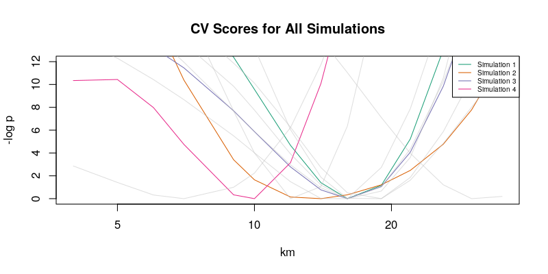 |
Figure 5: Cross-validation Scores for All Simulations
 |
 |
 |
 |
 |
 |
 |
 |
 |
 |
 |
 |
 |
 |
 |
 |
 |
 |
 |
 |
 |
 |
 |
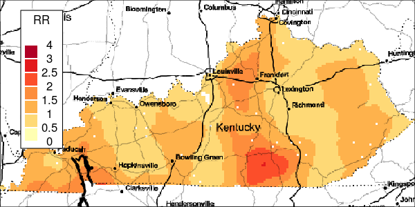 |
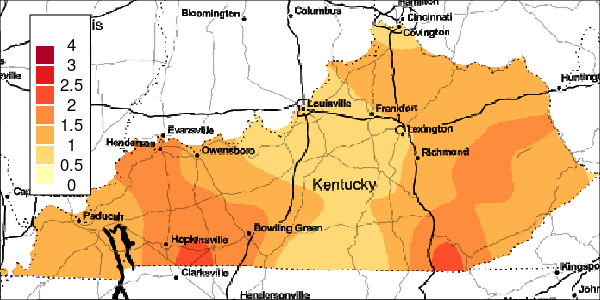
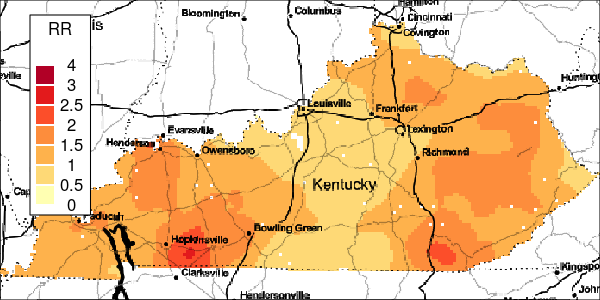
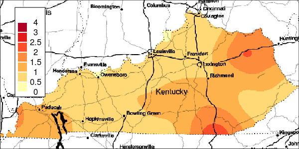
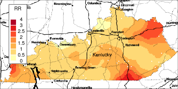
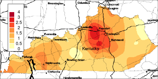
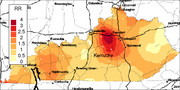
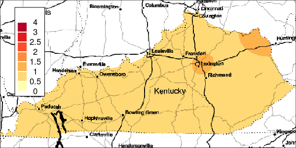
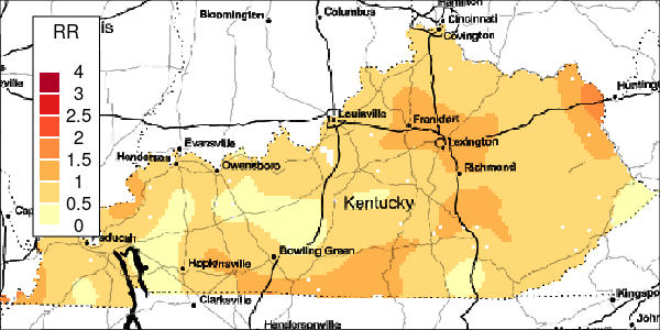
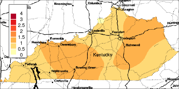
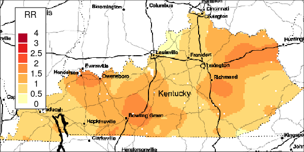
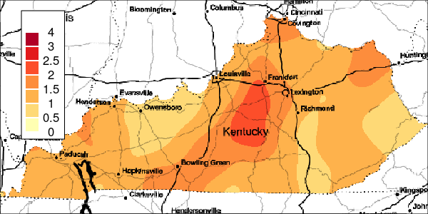
Figure 6: Estimated and True Relative Risk
Nguyen P, Brown PE, Stafford J. Mapping cancer risk in southwestern Ontario with changing census boundaries. Biometrics. 2012; 68(4): 1229-37.
Besag J, York J, Mollie A. Bayesian image restoration, with two applications in spatial statistics. Ann Inst Statist Math. 1991; 43(1): 1-59.